5 Reporting

# load data
load(url('https://github.com/systats/workshop_data_science/raw/master/Rnotebook/data/ess_workshop.Rdata'))
# filter data

library(dplyr)
ess_ger <- ess %>%
  dplyr::filter(country == "DE") %>%
  mutate(age2 = age*age)

fit0 <- lm(imm_econ ~ 1, data = ess_ger)
fit1 <- lm(imm_econ ~ left_right + vote_right, data = ess_ger) 
fit2 <- lm(imm_econ ~ left_right + vote_right + edu + age + gender, data = ess_ger)

5.1 Tabellen

5.1.1 stargazer

library(stargazer)
stargazer(list(fit0, fit1, fit2), type = "html")


	Dependent variable:

	imm_econ
	(1)	(2)	(3)

left_right		-0.187^***	-0.174^***
		(0.024)	(0.024)

vote_right1		-1.985^***	-1.991^***
		(0.226)	(0.224)

edu			0.162^***
			(0.020)

age			-0.004^*
			(0.002)

genderMale			0.335^***
			(0.086)

Constant	5.831^***	6.745^***	5.841^***
	(0.044)	(0.112)	(0.185)


Observations	2,817	2,740	2,721
R²	0.000	0.059	0.087
Adjusted R²	0.000	0.058	0.086
Residual Std. Error	2.335 (df = 2816)	2.253 (df = 2737)	2.221 (df = 2715)
F Statistic		85.459^*** (df = 2; 2737)	52.031^*** (df = 5; 2715)

Note:	p<0.1; p<0.05; p<0.01

5.1.2 texreg

library(texreg)
screenreg(list(fit0, fit1, fit2))

## 
## ==================================================
##              Model 1      Model 2      Model 3    
## --------------------------------------------------
## (Intercept)     5.83 ***     6.74 ***     5.84 ***
##                (0.04)       (0.11)       (0.18)   
## left_right                  -0.19 ***    -0.17 ***
##                             (0.02)       (0.02)   
## vote_right1                 -1.98 ***    -1.99 ***
##                             (0.23)       (0.22)   
## edu                                       0.16 ***
##                                          (0.02)   
## age                                      -0.00    
##                                          (0.00)   
## genderMale                                0.33 ***
##                                          (0.09)   
## --------------------------------------------------
## R^2             0.00         0.06         0.09    
## Adj. R^2        0.00         0.06         0.09    
## Num. obs.    2817         2740         2721       
## RMSE            2.34         2.25         2.22    
## ==================================================
## *** p < 0.001, ** p < 0.01, * p < 0.05

#texreg(list(fit0, fit1, fit2))
#htmlreg(list(fit0, fit1, fit2))

5.1.3 sjPlot

viele weitere Einstellungsmöglichkeiten findest du hier.

library(sjPlot)
sjt.lm(fit0, fit1, fit2, use.viewer = F, show.ci = F, show.se = T)

	imm_econ			imm_econ			imm_econ
	B	std. Error	p	B	std. Error	p	B	std. Error	p
(Intercept)	5.83	0.04	<.001	6.74	0.11	<.001	5.84	0.18	<.001
left_right				-0.19	0.02	<.001	-0.17	0.02	<.001
vote_right (1)				-1.98	0.23	<.001	-1.99	0.22	<.001
edu							0.16	0.02	<.001
age							-0.00	0.00	.065
gender (Male)							0.33	0.09	<.001
Observations	2817			2740			2721
R² / adj. R²	.000 / .000			.059 / .058			.087 / .086

sjt.lm(fit0, fit1, fit2, 
       use.viewer = F,
       show.std = TRUE,  
       show.ci = F)

imm_econ

std. Beta

(Intercept)

5.83

<.001

6.74

<.001

5.84

<.001

left_right

-0.19

-0.15

<.001

-0.17

-0.14

<.001

vote_right (1)

-1.98

-0.17

<.001

-1.99

-0.17

<.001

edu

0.16

0.15

<.001

age

-0.00

-0.03

.065

gender (Male)

0.33

0.07

<.001

Observations

2817

2740

2721

R² / adj. R²

.000 / .000

.059 / .058

.087 / .086

5.2 Show me your model!

With the sjp.lm function you can plot the beta coefficients with confidence intervals as so called “forest plots”.

Als nächstes werden wir fast auschließlich auf das Package sjPlot zurückgreifen um unsere Modelle zu visualiseren.

5.2.1 Coefficient Plot (Forest)

type = "est" is default.

type = "est" Unstandardisierte \(\beta\) Koeffizienten ist voreingestellt.
type = "re" For multilevel random effect models.
type = "std" Standardisierte Koeffizienten \(\beta^*\).
type = "std2" Vorschlag von Gelman durch zwei Standardabweichungen zu Teilen zur besseren Vergleichbarkeit mit Dummies.

library(ggthemr)
library(ggplot2)
ggthemr("flat")

library(sjPlot)
plot_model(fit2)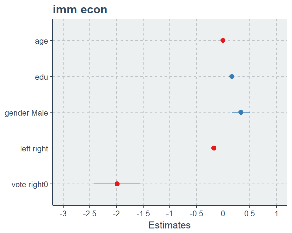

plot_model(fit2, vline.color = "red", sort.est = T)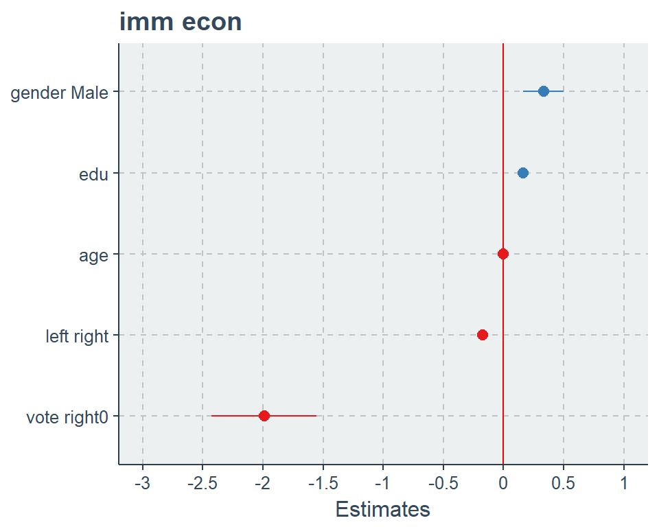

plot_model(fit2, show.values = TRUE, value.offset = .3, type = "std2")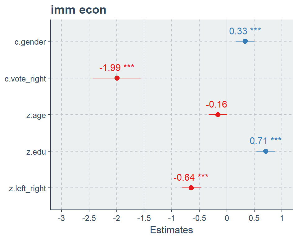

library(broom)
rbind(
  c("Nullmodel", glance(fit0)),
  c("Model 1", glance(fit1)),
  c("Model 2", glance(fit2))
)

##                  r.squared  adj.r.squared sigma    statistic p.value     
## [1,] "Nullmodel" 0          0             2.33521  NA        NA          
## [2,] "Model 1"   0.0587767  0.05808893    2.253388 85.45891  9.963587e-37
## [3,] "Model 2"   0.08744187 0.08576128    2.221265 52.03058  1.115144e-51
##      df logLik    AIC      BIC      deviance df.residual
## [1,] 1  -6385.753 12775.51 12787.39 15356.23 2816       
## [2,] 3  -6112.462 12232.92 12256.59 13897.82 2737       
## [3,] 6  -6029.495 12072.99 12114.35 13395.86 2715

5.2.2 Marginal Effects

sjp.lm(fit2, type = "eff")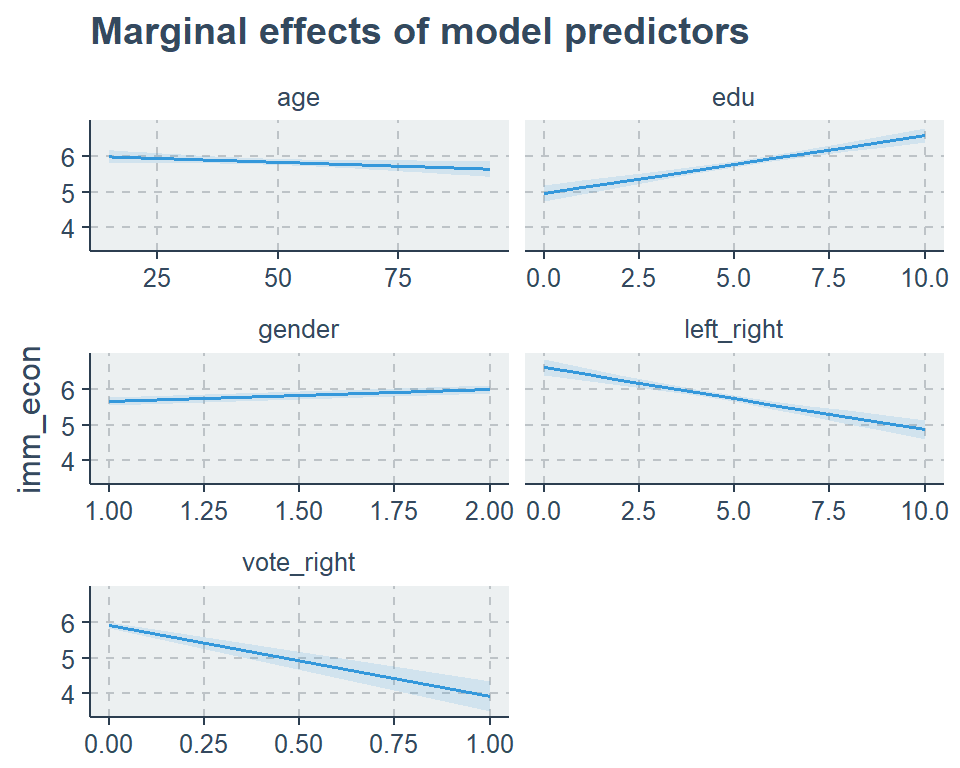

sjp.lm(fit2, 
       type = "eff", 
       facet.grid = F, 
       vars = "left_right")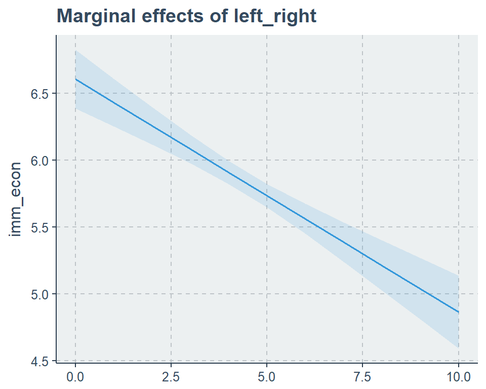

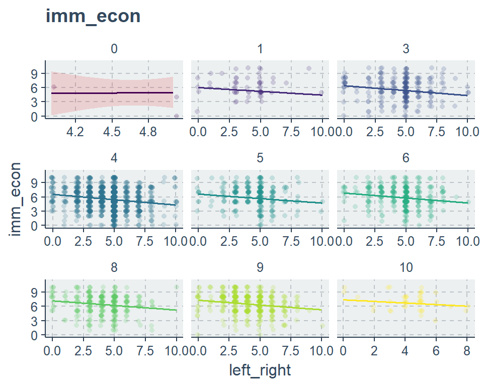
5.2.3 Predicting values

sjp.lm(fit2, type = "pred", vars = "left_right", point.alpha = .1)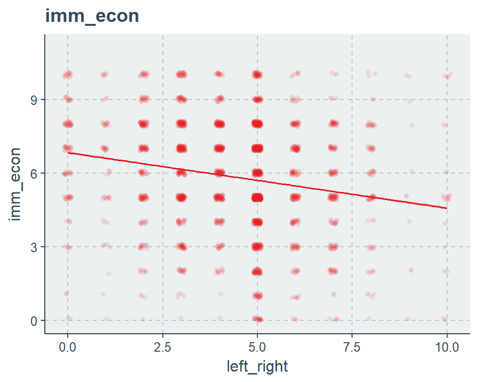

sjp.lm(fit2, type = "pred", vars = c("left_right", "edu"))$plot +
  viridis::scale_color_viridis(discrete = T)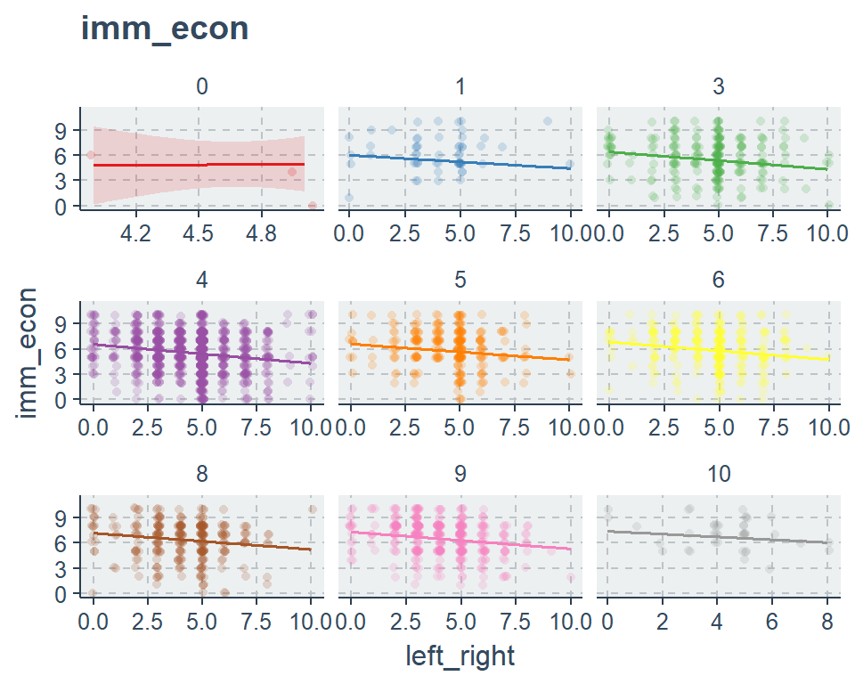

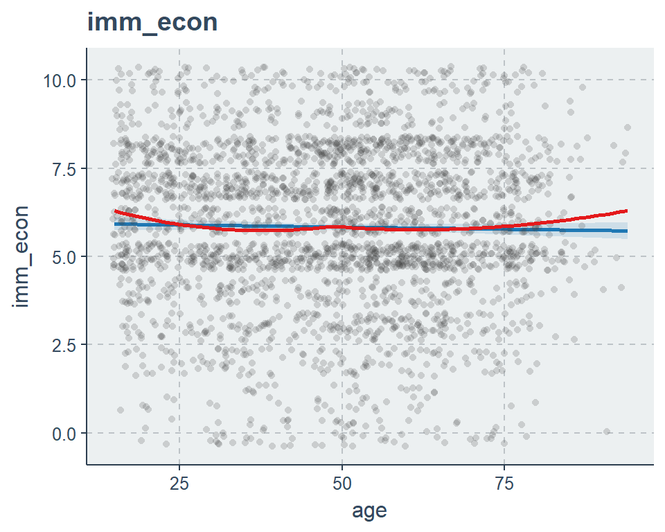
sjp.lm(fit2, type = "slope", show.loess = TRUE, vars = "age")